In this series of blog posts, we discuss work done to port the COVID-19 Dynamic Causal Model (DCM) to Octave, an open source tool. While this project was conceptually simple (especially given the strong similarity between the two languages we are concerned with, MATLAB and Octave), its implementation proved surprisingly difficult in practice. Where our other blog posts have discussed an overview of the problem and the theory of DCMs, in this blog post we look at the practicalities that realizing this project entailed.

In the first part of this blog, we provide some more details on the motivation and setup of the project we’ve undertaken. The current state of the code is not extensively modifiable, so we also provide some guidance for interested users to experiment with the implemented DCM. If you’re most interested in getting involved with this and your hands dirty with the code, you might want to skip to the next section, or go straight to the project repository.

SPM, DCM and Open Source

Dynamic Causal Modelling is a modelling tool out of neuroimaging, originally designed for modelling relationships between brain regions on the basis of FMRI scans, and later expanded to other paradigms. Within this field, Dynamic Causal Modelling has seen very wide success and citation, and in many respects is one of the states of the art in neuroimaging analysis.

However, while Dynamic Causal Modelling has generally remained within the neuroscience ecosphere, the technique itself is theoretically a very general and powerful time series modelling technique. Notably, as we discuss in our other blog post, Dynamic Causal Modelling is an explainable, causative and generative technique that effectively infers the whole space of possible solutions (and their likelihoods) at once, that has advantages over several other similar techniques. Most recently, Dynamic Causal Modelling has been applied with some success to modelling the COVID-19 pandemic.

Currently, the most widely used implementations of DCMs exist inside the SPM12 neuroimaging toolbox. SPM12 is open source software maintained by the Functional Imaging Laboratory under the Wellcome Trust and implemented in the MATLAB programming language. The source code for SPM (and the DCM for COVID-19 model contained within) is open source under a GPL-2 License. GPL-2 license is a copyleft license; the source code of any GPL-2 licensed software that is distributed must be made available on request, and any software that is distributed and makes use of GPL-2 licensed code (or derivatives of it) must also be GPL-2 licensed.

Unfortunately, while it is excellent that the SPM12 software is provided as free and open source, the current MATLAB dependent implementation means that, in practice, the software is fully dependent on proprietary, closed sourced code to run. To be fair to the SPM12 team, they do try to provide Octave (see below) compatibility where possible, but this is very much a second class citizen and for some of the more complicated parts (such as some of the DCM implementations), functionality is patchy. This presents several problems.

The first and most obvious problem is that, being proprietary software, one must pay for a MATLAB license, which is not always cheap. However, many using this software will already have a license through their institution, or feel that the price is simply the cost of doing business.

A more pressing concern for many is the risk of placing a central point of failure, and one on a commercial entity. The software essentially exists only as long as MATLAB exists as an entity, and as long as MATLABs licensing conditions remain compatible with the SPM12 project. Oracle, in a similar situation, is rather (in)famous for being litigious), and imposing restrictive constraints on licensing for it’s version of Java. Mathworks have not faced as much criticism around their business practices as oracle, but have still taken a strong stance on competition to it’s MATLAB tooling in the past.

Fortunately, alternatives do exist to MATLAB. There are, for example, many programming languages that Dynamic Causal Modelling could be re-implemented in that would be entirely free and open source (Python, R, C++). However, there is one particular standout among alternatives to MATLAB in GNU Octave. GNU Octave is a project that implements a language so close to MATLAB that the two are (almost) entirely interoperable – code written in MATLAB can run (almost) unchanged in Octave and vice-versa. This provides the possibility of an implementation that provides a strong offset to the risks set out above, without compromising the existing functionality.

This brings us to the goal of the current project, which is to implement a standalone subset of the Dynamic Causal Modelling functionality of SPM in Octave in a way that is also backward compatible with MATLAB. Note that we specify a standalone subset. This is because the SPM project as a whole is extremely large, and a full port would be a truly substantial undertaking. In keeping with contemporary topics, we chose to port the DCM model of the COVID-19 pandemic.

As we will see in later sections, while the similarities between Octave and MATLAB make this project theoretically very simple, it’s practical realization was not quite as easy as we expected. One of the goals of this blog post is to discuss the challenges we faced, not only because they are interesting in and of themselves, but also to provide guidance to others exploring similar problems.  A point we will particularly focus on is how further work might be done to extend or explore the existing code. Before this though, we provide a high level overview of the code ported, to give this discussion context.

DCM for COVID-19 Standalone

In this section we provide a high level overview of the implementation of the DCM for COVID-19 standalone. While not necessary, we suggest that many readers will benefit from reading this while looking at, and perhaps experimenting with the code. To get a working version of the project code, follow the steps below:

Install

1. Install Octave (or MATLAB)
2. Clone the repo
3. That’s it

Run

1. Navigate to the top level directory of the repository
2. In Octave, run the command DEM_COVID();
3. A full run will take in the region 1-2 hours in MATLAB and 6-12 in Octave

Run tests (optional)

1. Navigate to the top level directory of the repository
2. In Octave, run the command DEM_COVID_tests();
3. Tests should take in the region of 10 minutes to execute, and report success in all tests when done

Looking at a brief overview of the repository, it’s worth making two comments to those not familiar with MATLAB and Octave as programming languages. The first is that in Octave and MATLAB, each global function must be implemented in its own separate file. This, combined with the fact that SPM implements quite a lot of its own baseline functionality, means that the repository containing the standalone DCM ends up very populated. This doesn’t necessarily reflect an overly complicated program structure and, indeed, we won’t discuss most of these individual files. The second note is in terms of program structure. The SPM software from which we have ported our standalone follows many other MATLAB and Octave programs in making extensive use of the Struct data structure as a way of passing and manipulating data. Data is generally accumulated and stored in these structs, which are passed to functions. This way of working very loosely resembles some aspects of object oriented programming. With these notes aside, the structure of the COVID-19 DCM is fairly simple and can be seen in the annotated Figure 1.

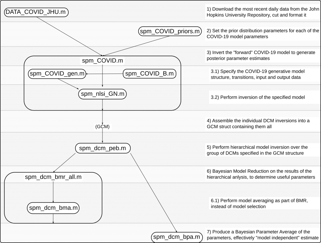
Up to date real world COVID-19 data is imported from the DATA_COVID_JHU function, and formatted for further processing. The data for each individual country is passed separately to the SPM_COVID.m function. This takes the countries data, a generative model specified by spm_COVID_gen (with transition matrix specified by spm_COVID_B) and priors specified by spm_COVID_priors and creates a model that it calls the spm_nlsi_GN.m function to invert.

This produces a DCM for each country, which is then assembled into the GCM cell array, containing all countries. This GCM cell array is then passed to the spm_dcm_peb.m function, which estimates a hierarchical model across all countries. This is one of the useful end results of the routine.

There are two outputs from this hierarchical model, a GCM array containing the hierarchical dynamic model, and a DCM array containing individual first level models. We analyze the usefulness of the parameters of this model using Bayesian Model Reduction, using the spm_dcm_bmr_all.m function (which calls spm_dcm_bma.m). The DCM array the individual first level models with empirical parameter estimates. We generate a “model free” estimate of parameters across these models using Bayesian parameter averaging using the spm_dcm_bpa.m function.

Discussion

Realizing the implementation above in a form compatible with MATLAB and Octave is, in theory, not an overwhelmingly difficult task. The extremely high compatibility between MATLAB and Octave means that the vast majority of the work is simply finding the relevant bits of code in SPM12, and tweaking any small inconsistencies in e.g. syntax.

One of the challenges we faced in this respect was the SPM12 project itself. Without detracting from the excellent work that contributors to the SPM software have done in providing an amazing tool, it’s fair to say the software could be more comprehensively structured and thoroughly documented. To quote from John Griffiths who seems to have tried to tackle a very similar problem to the one covered in this blog post:

“DCM lives inside SPM [a neuroscience toolbox], somewhat confusingly spread across multiple sub-toolboxes, and following the standard SPM convention of being cryptically coded and poorly (if at all) documented”

In fairness to SPM, this situation does seem to have markedly improved in the last few years, and was not too egregious for our particular task (the COVID-19 DCM). Nonetheless, we found that while it was often not too bad to find where a missing function to be ported was located, it was often difficult to understand exactly what it was doing, and where it fitted into the greater SPM (or DCM) software architecture.

Another interesting challenge we faced is that while Octave and MATLAB are very similar, they are not quite identical. While some of these differences are at the level of syntax (e.g., it’s possible to write a case statement that works in Octave but not MATLAB), more problematic differences arise in the implementation (or lack thereof) of baseline functionality. MATLAB development has generally advanced at a substantially faster rate than Octave, and certain functionality exists (and is used in SPM for example) that simply doesn’t exist, or behaves differently, in Octave. Particularly notable cases of this are in FileIO, in which Octave behaves vastly differently to MATLAB when importing files. This different behaviour was a source of many problems for us, especially in the case of FileIO which introduced some rather subtle and insidious bugs. Though not a huge problem in SPM itself, which has generally avoided using some of MATLABs later features in order to keep compatibility with older versions, newer versions of MATLAB implement paradigms that simply don’t exist in Octave. Octave does, for example, not have the same functionality with respect to Strings as MATLAB does, and one must actually be quite careful in their use of single (‘) versus double (“) quotes when writing code to make sure code works in both languages.

One particularly interesting case of divergence between MATLAB and Octave that deserves it’s own special discussion is that the two languages fundamentally compute slightly different results for some floating point operations. This difference is trivially small for any individual operation, but when certain types of operations are stacked up, these differences can become large enough to be significant. In isolation, this error is small, and is unlikely to result in any qualitative changes in behavior. In the context of model inversion however, a lot of (for example) numerical differentiations occur, ultimately elevating what can start out as a small error to something more significant. As we discuss below, this also makes some difficulty in writing tests that are consistent across the two languages.

Testing itself was also something of a challenge. We weren’t able to get the inbuilt tests inside SPM working (due to, we think, missing some test data), and on closer inspection we felt that they didn’t have sufficient coverage and depth to warrant the substantial effort of re-implementation. Writing a testing suite consistent with both languages was also a challenge. MATLAB and Octave implement completely different testing frameworks, with little compatibility between the two. MATLAB implements an xunit-like testing framework, while Octave uses BIST testing. In order to make a testing framework that would work in both, we ended up building a simple testing framework from scratch. Given the floating point issues above, these tests were built with some leeway in the numerical comparisons.

Despite some of these interesting challenges, we had quite a good time with this project. The similarities between Octave and MATLAB smoothed over a lot of the difficulties, and this particular part of the SPM12 project was quite self-contained and well documented compared to other parts. One open issue with the software as it stands is how to customize and explore the models that it develops. We initially didn’t explore this in great detail, but we think this will be of interest to most readers so we now engage with and discuss this topic.

Customizing the Model

There is currently not much scope within the model to easily experiment and many interesting changes need to be made at the level of modifying code rather than anything simpler. Here we cover some simple examples of some common changes a user might wish to experiment with.

Note that there is no guarantee of model stability if any of these changes are made: insofar as substantial changes are made to the model, there is an equally substantial chance that the model will not work.

Modifying a variables prior

One might wish to modify the priors used in the model. There are two axes we can do this on for each variable, the variable’s expectation and it’s (co) variance. Note that setting either of these to zero (or close to) may cause unwanted effects, see “fixing a variable” and “removing a variable”. For example, if we wished to change out initial estimation of the number of contacts as work, we could change (in spm_COVID_priors.m) from:

P.Rin = 4;                    % effective number of contacts: home
To:
P.Rin = 5;                    % effective number of contacts: home

Fixing a variable

To fix a variable at a certain value, in theory we set the prior expectation of that variable to our chosen value, and its prior (co)variance to zero. In practice, actually setting variance to zero causes practical problems with some functions, so we simply set it to a very small value (1e-03). For example, if we wished to fix out the effects of social distancing, we could change the covariance of the social distancing exponent (in spm_COVID_priors.m) from:

C.sde = W;                    % social distancing threshold
To:
C.sde = 1e-3;                    % social distancing threshold

Adding or Removing a variable

One way to remove a variable is to set it at a value where it has no effect, and fix it’s value there by setting the prior covariance to a small number (see instructions above). In practice, finding such a value might be difficult or impossible. If this isn’t possible, then the process for removing a variable is exactly the inverse as the instructions for adding one, which we cover now.

Adding a variable is slightly more involved in the previous steps, all of which could be achieved by modifying the priors of the model. Adding a variable necessitates changes to the model structure itself. Depending on the variable we’re adding, changes must be made to all of spm_COVID_priors.m, spm_COVID_B.m files, and (perhaps) spm_COVID_gen.m.

Suppose we wish to add a variable “Blorg”, modelling the effect of a popular new game “Blorg” that is inciting people to stay at home instead of going to work. To model Blorg, we’d have to make the following changes:

We’d have to modify our transition matrix function spm_COVID_B.m to take Blorg into account. We’d want to change the probability of transitioning to work from home. The relevant bit of the code would be to change (in spm_COVID_B.m) from:

Pout = Psde*P.out;                   % P(work | home)
To:
Pout = Psde*P.out*Blorg;                   % P(work | home)

We also need to set Priors for Blorg. Blorg is very popular, so we’re going to estimate a-priori that it will cut work attendance in half, and that this estimate is of “high” precision (so covariance is W=1/256). We also need to specify Blorg on the list of named variables. We can do this by adding the following lines to spm_COVID_priors.m:

P.Rin = 0.5;
C.sde = W;
names{28} = ‘blorg’;

In this case, Blorg only affects the model through transition probabilities and so we don’t need to change spm_COVID_gen.m. For now, we will leave out changes to spm_COVID_gen, as it’s unlikely that these will be needed in general.

Conclusion

This work was part of a greater project by Embecosm to make the UCL model of the COVID-19 pandemic truly Free and Open Source. We discussed the practical implementation of the Dynamic Causal Modelling code, walked through its architecture and provided some examples for users to modify the code. Those interested in the theory underlying this all may find our other blogpost of interest.

The rest of this blog post is dedicated to a “key functions”  appendix, which provides some more detail on the functionality of each of the major functions discussed in the architecture section (and shown in the architecture diagram).

 

Key functions

The key functions in realising the COVID-19 DCM, modelling in Figure 1. This is broadly adapted from the documentation provided within SPM12, with some updates and some omissions fixed.

DEM_COVID.m

Central function that runs the COVID-19 Analysis. Caller of all functions below.

Inputs: NA

Outputs: NA

DATA_COVID_JHU.m

Download and import function of up-to-date COVID data. Pulls from a github repository provided by John Hopkins University, which is updated daily with COVID pandemic data, and processes it into a suitable format to be operated on by later functions.

This function (especially in Octave) is very much tuned for the data as formatted in this specific github repository, and is unlikely to work on any others.

Inputs:

• n – the number of countries to retain in the dataset (default 16)

Outputs:

• data – struct containing formatted data from the n countries.
  • Fields:
  • data(k).country – country
  • data(k).pop     – population size
  • data(k).lat     – latitude
  • data(k).long    – longitude
  • data(k).date    – date when more than one case was reported
  • data(k).cases   – number of cases,  from eight days prior to first cases
  • data(k).death   – number of deaths, from eight days prior to first cases
  • data(k).recov   – number recovered, from eight days prior to first cases
  • data(k).days    – number of days in timeseries
  • data(k).cum     – cumulative number of deaths

spm_COVID.m

Model inversion for the COVID-19 Model. Mostly specifies a few COVID-19 specific DCM parameters then calls the generic DCM inversion function spm_nlsi_GN.m to do the actual inversion itself.

Inputs:

• Y   – time series data
• pE  – prior expectation of parameters
• pC  – prior covariances of parameters
• hC  – prior covariances of precisions

Outputs:

• F   – log evidence (negative variational free energy)
• Ep  – posterior expectation of parameters
• Cp  – posterior covariances of parameters
• pE  – prior expectation of parameters
• pC  – prior covariances of parameters
• Eh – posterior log-orecisions

spm_nlsi_GN.m

Generic routine for inverting a DCM model, using expectation maximisation to find the maximised free energy, and the related estimates of the posterior probability distribution functions of the parameters of the DCM.

Inputs:

• M – Model structure
  • M.G (or M.IS) – function name f(P,M,U) – a generative model. Specifies the dynamical systems model of the system to be inverted. Defaults to the spm_int function (not implemented in the standalone) if no option is specified. In the COVID-19 DCM, we specify this as spm_COVID_gen, the function which specifies our COVID-19 dynamical system.
  • M.FS – function name f(y,M)   – feature selection. This [optional] function performs feature selection.
  • M.P  – starting estimates for model parameters [optional]
  • M.pE – prior expectation      – E{P}   of model parameters
  • M.pC – prior covariance       – Cov{P} of model parameters
  • M.hE – prior expectation      – E{h}   of log-precision parameters
  • M.hC – prior covariance       – Cov{h} of log-precision parameters
• U – Input structure
  • U.u  – inputs (or just U)
  • U.dt – sampling interval
• Y – Output structure
  • Y.y  – outputs (samples (time) x observations (first sort) x …)
  • Y.dt – sampling interval for outputs
  • Y.X0 – confounds or null space      (over size(y,1) samples or all vec(y))
  • Y.Q  – q error precision components (over size(y,1) samples or all vec(y))

Outputs:

• Ep  – (p x 1)         conditional expectation    E{P|y}
• Cp  – (p x p)         conditional covariance     Cov{P|y}
• Eh  – (q x 1)         conditional log-precisions E{h|y}
• F   – [-ve] free energy F = log evidence = p(y|f,g,pE,pC) = p(y|m)

 

• L – Components of F. Optional, not used in the COVID-19 DCM.
• dFdp – Gradient. Optional, not used in the COVID-19 DCM.
• dFdpp – Curvature. Optional, not used in the COVID-19 DCM.

 

spm_COVID_gen.m

Generative model for the COVID-19 DCM. Generates predictions and hidden states of a COVID model. Used by spm_COVID.m as the generative function for model inversion.

Inputs:

• P – model parameters
• M – model structure (requires M.T – length of timeseries)
• U – number of output variables [default: 2] or indices e.g., [4 5]

Outputs:

• Z{t} – joint density over hidden states at the time t
• Y(:,1)  – number of new deaths
• Y(:,2)  – number of new cases
• Y(:,3)  – CCU bed occupancy
• Y(:,4)  – effective reproduction rate (R)
• Y(:,5)  – population immunity (%)
• Y(:,6)  – total number of tests
• Y(:,7)  – contagion risk (%)
• Y(:,8)  – prevalence of infection (%)
• Y(:,9)  – number of infected at home, untested and asymptomatic
• Y(:,10) – new cases per day
• X       – (M.T x 4) marginal densities over four factors
  • location   : {‘home’,’out’,’CCU’,’morgue’,’isolation’};
  • infection  : {‘susceptible’,’infected’,’infectious’,’immune’,’resistant’};
  • clinical   : {‘asymptomatic’,’symptoms’,’ARDS’,’death’};
  • diagnostic : {‘untested’,’waiting’,’positive’,’negative’}

spm_COVID_priors.m

Specify the prior expectations and covariances of the COVID-19 generative models parameters. Used by spm_COVID.m to specify priors for the generative model.

Inputs:

• NA

Outputs:

• pE          – prior expectation (structure)
• pC          – prior covariances (structure)
• str.factor  – latent or hidden factors
• str.factors – levels of each factor
• str.outcome – outcome names (see spm_COVID_gen)
• str.names   – parameter names
• str.field   – field names of random effects
• rfx         – indices of random effects

spm_COVID_B.m

Specify the probability transition matrix for the COVID-19 DCM.

Inputs:

• x – probability distributions (tensor)
• P – model parameters
• r – marginals over regions

Outputs:

• T  – probability transition matrix

spm_dcm_peb.m

Perform hierarchical inversion across a group DCMs (or an individual DCM, see file for details). We specify the parameters to be considered as random (global) effects and those to be treated as fixed (local model specific) effects using the fields function.

Inputs:

• DCM    – {N [x M]} structure array of DCMs from N subjects
  • DCM{i}.M.pE   – prior expectation of parameters
  • DCM{i}.M.pC   – prior covariances of parameters
  • DCM{i}.Ep     – posterior expectations
  • DCM{i}.Cp     – posterior covariance
  • DCM{i}.F      – free energy
• M – Model specification
  • M.X      – 2nd-level design matrix: X(:,1) = ones(N,1) [default]
  • M.bE     – 3rd-level prior expectation [default: DCM{1}.M.pE]
  • M.bC     – 3rd-level prior covariance  [default: DCM{1}.M.pC/M.alpha]
  • M.pC     – 2nd-level prior covariance  [default: DCM{1}.M.pC/M.beta]
  • M.hE     – 2nd-level prior expectation of log precisions [default: 0]
  • M.hC     – 2nd-level prior covariances of log precisions [default: 1/16]
  • M.maxit  – maximum iterations [default: 64]
  • M.Q      – covariance components: {‘single’,’fields’,’all’,’none’}
  • M.alpha  – optional scaling to specify M.bC [default = 1]
  • M.beta   – optional scaling to specify M.pC [default = 16] – if beta equals 0, sample variances will be used NB: the prior covariance of 2nd-level random effects is: exp(M.hE)*DCM{1}.M.pC/M.beta [default DCM{1}.M.pC/16] NB2: to manually specify which parameters should be assigned to which covariance components, M.Q can be set to a cell array of[nxn] binary matrices, where n is the number of DCM parameters. A value of M.Q{i}(n,n)==1 indicates that parameter n should be modelled with component i.
  • M.Xnames – cell array of names for second level parameters [default: {}]
• field – parameter fields in DCM{i}.Ep to optimise [default: {‘A’,’B’}] ‘all’ will invoke all fields. This argument effectively allows one to specify the parameters that constitute random effects.

Outputs:

• PEB – hierarchical dynamic model
  • PEB.Snames    – string array of first level model names
  • PEB.Pnames    – string array of parameters of interest
  • PEB.Pind – indices of parameters at the level below
  • PEB.Pind0 – indices of parameters in spm_vec(DCM{i}.Ep)
  • PEB.Xnames    – names of second level parameters
  • PEB.M.X – second level (between-subject) design matrix
  • PEB.M.W – second level (within-subject) design matrix
  • PEB.M.Q – precision [components] of second level random effects
  • PEB.M.pE – prior expectation of second level parameters
  • PEB.M.pC – prior covariance of second level parameters
  • PEB.M.hE – prior expectation of second level log-precisions
  • PEB.M.hC – prior covariance of second level log-precisions
  • PEB.Ep – posterior expectation of second level parameters
  • PEB.Eh – posterior expectation of second level log-precisions
  • PEB.Cp – posterior covariance of second level parameters
  • PEB.Ch – posterior covariance of second level log-precisions
  • PEB.Ce – expected  covariance of second level random effects
  • PEB.F – free energy of second level model
• DCM – 1st level (reduced) DCM structures with empirical priors. If DCM is an an (N x M} array, hierarchical inversion will be applied to each model (i.e., each row) – and PEB will be a {1 x M} cell array.

spm_dcm_bmr_all.m

Performs Bayesian Model Reduction on the given DCM (or cell array of DCMs). Performs (based on OPT), either selection of models among nested models of the specified DCMs, or Bayesian Model Averaging across them.

Inputs:

• DCM – A single estimated DCM (or PEB) structure:
  • DCM.M.pE  – prior expectation
  • DCM.M.pC  – prior covariance
  • DCM.Ep    – posterior expectation
  • DCM.Cp    – posterior covariances
  • DCM.beta  – prior expectation of reduced parameters (default: 0)
  • DCM.gamma – prior variance    of reduced parameters (default: 0)
• field      – parameter fields in DCM{i}.Ep to optimise [default: {‘A’,’B’}] ‘All’ will invoke all fields (i.e. random effects) If Ep is not a structure, all parameters will be considered
• OPT    – Bayesian model selection or averaging: ‘BMS’ or ‘BMA’ [default: ‘BMA’]

Outputs:

• DCM – Bayesian Model Average (BMA) over models in the final iteration of the search:
  • DCM.M.pE  – reduced prior expectation
  • DCM.M.pC  – reduced prior covariance
  • DCM.Ep    – reduced (BMA/BMS) posterior expectation
  • DCM.Cp    – reduced (BMA/BMS) posterior covariance
  • DCM.Pp    – Model posterior over parameters (with and without)
• BMR –  (Nsub) summary structure reporting the model space from the last iteration of the search:
  • BMR.name – character/cell array of parameter names
  • BMR.F    – free energies (relative to full model)
  • BMR.P    – and posterior (model) probabilities
  • BMR.K    – [models x parameters] model space (1 = off, 0 = on)
• BMA – Baysian model average (over reduced models; see spm_dcm_bma)

spm_dcm_bma.m

Bayesian model averaging procedure. Produces samples from a DCM posterior that are independent of any particular model.

Inputs:

• DCM   – {subjects x models} cell array of DCMs over which to average
  • DCM{i,j}.Ep – posterior expectation
  • DCM{i,j}.Cp – posterior covariances
  • DCM{i,j}.F  – free energy

Outputs:

• BMA   – Bayesian model average structure
  • BMA.Ep      – BMA posterior mean
  • BMA.Cp      – BMA posterior VARIANCE
  • BMA.F       – Accumulated free energy over subjects;
  • BMA.P       – Posterior model probability over subjects;
  • BMA.SUB.Ep  – subject specific BMA posterior mean
  • BMA.SUB.Sp  – subject specific BMA posterior variance
  • BMA.nsamp   – Number of samples
  • BMA.Nocc    – number of models in Occam’s window
  • BMA.Mocc    – index of models in Occam’s window

spm_dcm_bpa.m

Produce an aggregate DCM using Bayesian parameter averaging. Creates a new DCM in which parameters are averages over the number of fitted DCMs.

Inputs:

• DCM  – {N [x M]} structure array of DCMs from N subjects
  • DCM{i}.M.pE – prior expectations of P parameters
  • DCM{i}.M.pC – prior covariance
  • DCM{i}.Ep   – posterior expectations
  • DCM{i}.Cp   – posterior covariance
• nocd – optional flag for suppressing conditional dependencies. This is useful when evaluating the BPA of individual (contrasts of) parameters, where the BPA of a contrast should not be confused with the contrast of a BPA.

Outputs:

• BPA  – DCM structure (array) containing Bayesian parameter averages
  • BPA.M.pE – prior expectations of P parameters
  • BPA.M.pC – prior covariance
  • BPA.Ep   – posterior expectations
  • BPA.Cp   – posterior covariance
  • BPA.Pp   – posterior probability of > 0
  • BPA.Vp   – posterior variance
  • BPA….  – other fields from DCM{1[,:]}