At Embecosm, we have recently been taking an interest in time series modelling in the context of the COVID-19 pandemic and, in particular, the application of Bayesian methods to these problems.

In this blog post, we want to backtrack a bit and talk discuss how the Bayesian approach can fit into time series analysis in a more general sense, rather than just cutting edge COVID-19 modelling techniques. We’re going to do this by looking through a common time series modelling and forecasting technique, ARIMA (Auto-Regressive Integrated Moving Average), and how it compares with the somewhat similar Bayesian technique of Bayesian Structural Time Series (BSTS). We’re going to do this both with a discussion of the two techniques, and by providing some examples applying them to two interesting time series modelling cases.

There are really three messages we want to communicate with this post. The first is an introduction to ARIMA and BSTS, and a demonstration that our Bayesian method, BSTS, really isn’t difficult or hard to implement.  To help with this, code to perform the analysis and generate the plots below can be found in the Jupyter Notebook associated with this project here. The second thing we want to communicate is a comparison of the two methods , where the strengths and weaknesses of each lie. Finally, we want to show where these methods are limited, and what the ultimate driver for introducing more complicated techniques like the Dynamic Causal Modelling approach we explore previously is – the ability to account for extra information in our time series.

Background – Time Series Modelling

The scope of our modelling problem is a time series modelling problem and, in particular, a forecasting problem: predicting how a time series will evolve in future by observing it in the past.

Modelling data that is time-dependent presents us with some significant challenges. The cause of our difficulty is the presence of auto-correlation in time series data – that the value of my time point now is dependent on the value of some or all of my time points before. Auto-correlation presents problems to many of the tools and statistical methods we would usually wish to use which assume that our data points are independent from one another.

Independence is an assumption that is difficult to get away from. When our data are independent, we can create models by only considering our data-points themselves. When data are not independent however, we need to treat not only each data-point, but potentially it’s relationship to every other data-point as well. This can cause a rapid combinatorical explosion of factors under consideration, making whatever methods we’re interested in applying somewhere between difficult and impossible.

While we cannot often get ourselves into a situation in which we can leverage independence in time series modelling, it is often possible for us to insist that our time series data is stationary. A time series is stationary if the statistical properties of each time point in the series is constant. That is, that the mean, the variance, and the dependence relationship of each point with previous points remains constant through the whole time series. This is clearly a weaker assumption than independence, but still achieves a powerful and useful simplification.

There are three common properties or time series that we often stand in the way of stationarity. These are are trends, seasonality, and heteroscedasticity. A trend is a change in the mean over time. Heteroscedasticity corresponds to changing variance over time. Seasonality refers to regular recurring effects in the time series. In this blog, though heteroscedasticity is important, mots of our discussion will be concerned with trends and seasonality.

ARIMA

ARIMA (Auto-Regressive Integrated Moving Average) is a time series modelling technique that is capable of modelling stationary time series that are subject to trends (and, with extension, seasonality). ARIMA is really the union of three parts: “Auto-regresson”, “Integration” and “Moving Average”.

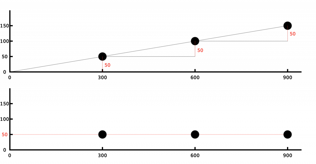
Let’s first discuss the Integration step. In this step, we de-trend our time series using the technique of differencing. Differencing works on the following observation: Though a time series with a trend has a non-constant mean, it’s rate of change (or rate of rate of change, etc.) may well be constant. We can attain this rate of change by looking at the difference between time points instead of the time points themselves. Given that doing this is a reversible process, this lets us produce (and analyse) a time series without a trend from a time series with a trend. Consider as an example the case of data with an upward, linear trend. The mean of these data will increase over time, but the difference between each data point will remain constant. This example is linear, but in general we can de-trend even fairly complicated relationships with iterative application of differencing.

When the data has been de-trended, we can apply the next step: auto-regression step can be applied. The auto-regressive step is, from the name, a regression of the time series on itself. In this case, it relates to us the current value of the time series to previous previous values (plus statistical error):

(1) Y_t = α + β₁Y_t-1 + β₂Y_t-2 + … + β_pY_t-p + ε_t

Where Y_t gives us the value of the time series now (at time t), Y_t-1 is the value of the time series one time step back, and so on. We can do this step because the time series is stationary: recall that one of the assumptions that stationarity makes is that the relationships between current and previous points in the time series should be fixed, as they are in the formula (1). We can fairly easily calculate the best (maximum likelihood) values of our unknown parameters Alpha and Beta using the ordinary least squares method we’d apply for a typical linear regression.

With the data de-trended, we can also perform the Moving Average part of the model. Here, instead of regressing on the previous values (as we did in the auto-regression step), we regress on previous errors.

(2) Y_t = α + Φ₁ε_t-1 + Φ₂ε_t-2 + … + Φ_qε_t-q

This too leverages our assumption that our time series is stationary, this time by assuming that the data points have a constant mean. The estimation of our optimal Φ values is significantly more complex than those in Auto-Regressive part of the model, as we can’t directly observe the ε we are interested in.

Each of these three parts of the ARIMA model that we have described above is dependent on a parameter. In the case f the auto-regressive step and the moving average step, these are p and q, which define the number of previous time steps we base our current time point estimates on. In the case of the differencing step, we define the parameters r, which defines the order of the differencing we will perform (differences, differences of differences, etc). The model can also be extended to tackle seasonality by adding 4 new parameters, P, Q, R and s. These are the equivalent ARIMA parameters for a seasonal effect across the data with period s.

Bayesian Structural Time Series

Bayesian Structural Time Series is a specific approach to solving “structural time series” models. A structural time series is a member of the very broad class of state-space models, which model our time series as observations of a hidden state that evolves over time. Specifically, this model states that our observations (y_t) of the real world that make up our time series are determined as a function of a hidden state (α_t) that evolves over time according to a Markov process (one in which each state is dependent only on the previous state).

A structural time series in particular posits a particular form for these relationships, that these functions between states and observations, and between states and previous states are linear subject to Gaussian noise. We can define our structural time series model with the paired equations:

(3) y_t = Z^T_tα_t + ϵ_t, ϵ_t ~ N(0, H_t)

(4) α_t+1 = T_tα_t + R_tη_t, ηt ~ N(0, Q_t)

We label (3) the observation equation because it links our hidden state to our observed state and we label (4) the transition equation, because it links each internal state to each previous internal state. Many different models can be expressed in this form, including the ARIMA model described above.

Expressing our model using (3) and (4) is a very useful thing to do because we can build up the matricies Z^T_t and T_t that govern how our model evolves in a modular fashion that lends itself to easy interpretation. Consider, for example, the “basic structural model” (plus regression) dictated by (equations 5-8) consisting of three components, a trend, seasonality (as in ARIMA) and a regression component (not seen thus far). A regression component is one that predicts the value of a time series based on the value of a related one, for example we might based our prediction of an electricity usage at a given time based partially on time series of outside temperature at the same time.

(5) y_t = μ_t + τ_t + β^Tx_t + ϵ_t (Observation and regression)

(6) μ_t+1= μ_t+ δ_t-1 + u_t (Level and trend)

(7) δ_t+1 = δ_t+ v_t (Level and trend)

(8) τ_t= – ∑ τ_t-s + w_t (Seasonal)

Each of the components we’re modelling has a natural interpretation that can be clearly written out in the form above, which can also be expressed in (3) and (4). Finding a solution for these models is more involved than the ARIMA approach. Eschewing an extensive explanation inappropriate for the short form of this post, we can summarize the process of finding our solutions in three parts:

1) Kalman filtering, a recursive approach that iterates along our time series, updating an estimate of our parameters at each step

2) The use of Bayesian slab-and-spike priors to select the “best” regression components

3) Combining the results of the above two using Bayesian Model Averaging

The Bayesian namesake of this method comes from the fact that all these steps speak to a natural Bayesian formulation of the problem, though Kalman filtering is by no means a strictly Bayesian technique, also having a very nice “classical” formulation.

Applications

As we said at the start, one of the ways we’re looking to compare these two techniques is by looking at example of each of these techniques over two datasets – electricity forecasting and stock market data. We’ve picked these datasets to show both the strengths of these two techniques, and demonstrate the cases in which (both of) these types of approaches are fundamentally limited. Our first example, our electricity datasets, is one that is ideally suited for these types of analysis. The data is reasonably easy to de-trend, shows strong seasonality, and previous data points are excellent predictors of future ones. As we will see, both techniques perform fairly well (both qualitatively and quantitatively) at making predictions on this set.

Our stock market data, on the other hand, is a significantly more difficult beast. It is fairly well known that, despite the presence of long term trends, stock market data essentially moves as a random walk (shortly, a process in which the mean of each data point is the previous) in the short term. This means that while this data is theoretically well suited for analysis with, for example, ARIMA, in that is is very easy to convert to a stationary process, it is also rather difficult to make strong predictions. We show an exemplar of one approach to mitigate this problem (albeit one with limited use the problem we’d be really interested in, forecasting), using regression.

One issue we have circumvented in our discussion of our two techniques to this point is the model selection problem – we have broadly described how our ARIMA and BSTS models work, and how they are parameterized, but not how to choose between different candidates parameters. For example, how do I determine which values of p, q and r I should select in my ARIMA model? To keep this post short, on topic, and simple we’re going to avoid this discussion. Shortly, for those reading this post who are not familiar with how to approach these problems, the solution is generally to use cross-validation, and in this case, likely with reference to ACF/PACF plots as sanity checks.

Electricity Data

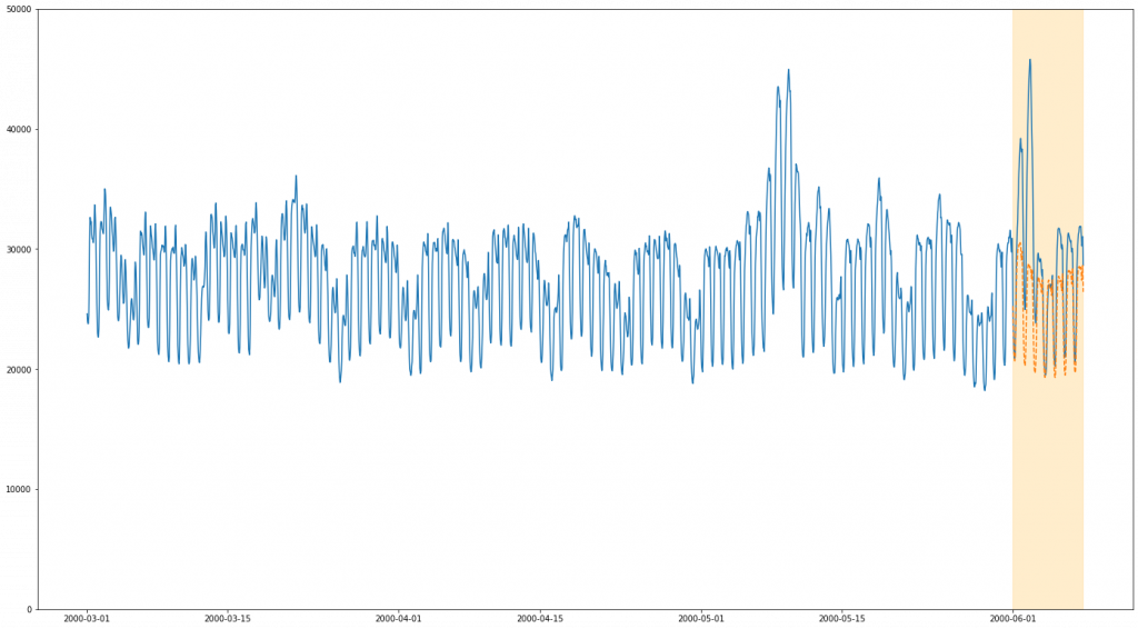
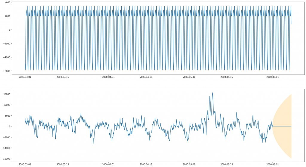
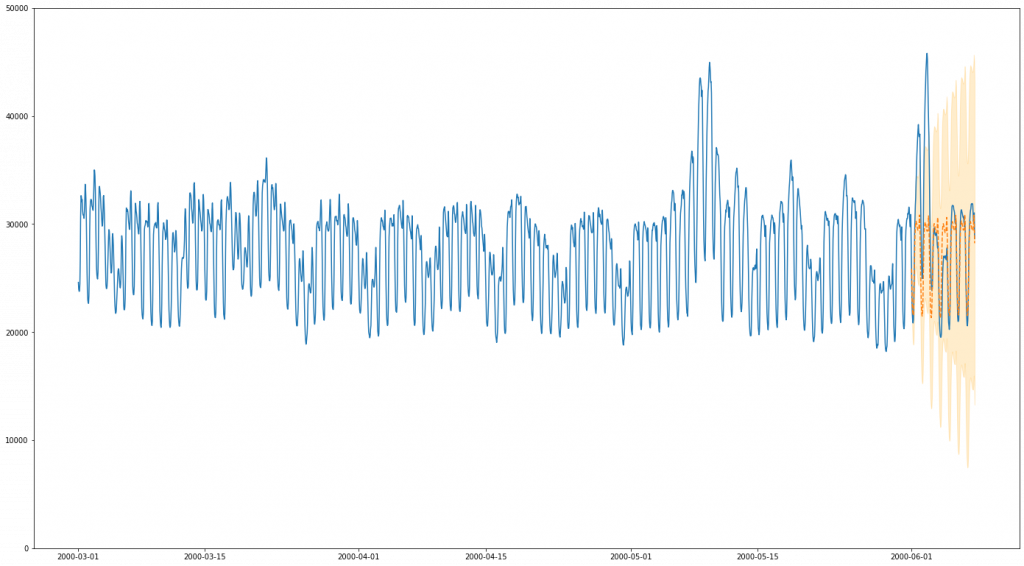
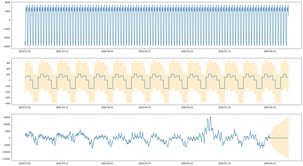
Our first dataset is our “easy” dataset – electricity usage from PJM (A US electiricity company).  One interesting part of this dataset is the issue of multiple seasonality. The ARIMA methods as described above only really provisions for one level of seasonality, for example a seasonal effect of the time of day. In this dataset, there is compelling reason to believe that data doesn’t just vary seasonally according to the time of day, but also according to the day of the week (and, if we examined the plots over a wider period, likely over month of the year. It is possible to extend ARIMA to account for multiple seasonality, but it is significantly non-trivial. With BSTS this is much less of an issue, as multiple seasonality simply becomes multiple seasonal “components”. Here, we opt to do one run of our ARIMA model and two runs of our BSTS model to compare the two. Our first BSTS model will be one that matches the seasonality of our ARIMA model (modelling daily periodicity), and the second one that extends it with a second seasonal effect – weekly periodicity.

Code to perform the analysis and generate the plots below can be found in the Jupyter Notebook associated with this project here.

ARIMA

BSTS

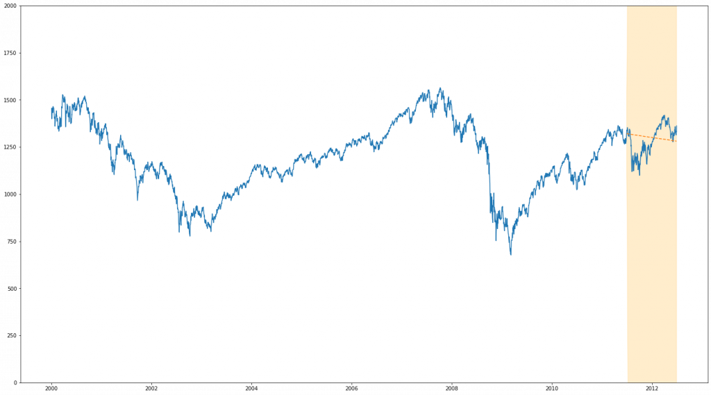
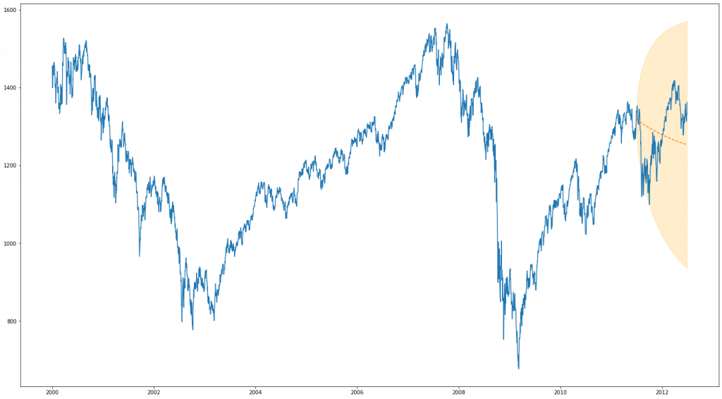
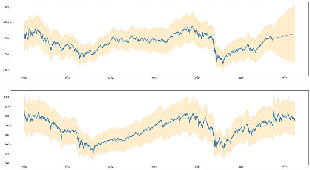
Stock Market Data

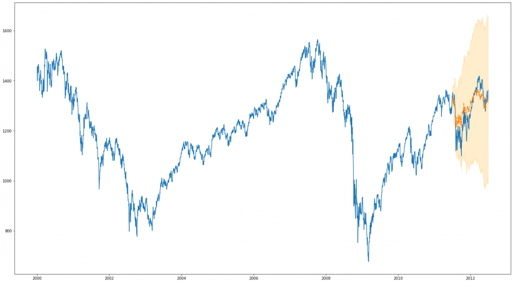
We now look at our hard dataset. As we’ve previously discussed, we expect to have very little seasonality or auto-correlation in our plots. What we are really running into here is a fundamental limitation of our approach – in this instance there is simply only a very limited amount of information given by previous prices in respect of future ones. One way we can circumvent this problem and improve our predictive power is to base our estimate on other things that are correlated with out measure of interest. One tool we can use to do this in the context (albiet one with limited use in forecasting) of both BSTS and ARIMA is to make use of a regression term, basing our estimated outcome partially from a correlated time series. In this case, we choose to use a highly correlated FTSE100 stock price dataset. This gives us much more information to work with and, as we’ll see, substantially improves our results.

Code to perform the analysis and generate the plots below can be found in the Jupyter Notebook associated with this project here.

ARIMA

BSTS

Discussion

We’ve talked through our techniques and applied them to a few interesting problems, now let’s discuss the takeaways from of all of this.

The first discussion we’d often have around these techniques is the relative performance of the two – which is the better predictor. In this blog post, this is (unusually) perhaps the least important discussion of all. Insofar as we have been able to compare like with like, the two methods have performed very similarly, with BSTS perhaps fractionally inching ahead in performance on our dataset when comparing multiple seasonality versus ARIMA single seasonality. Though the results we get are interesting, ultimately, in our examples we were not tuning either of our methods to the cutting edge to try and extract the best performing one, instead focusing on providing good examples. Any difference between the two can only really be weakly indicative. That said, overall, BSTS did perform slightly better, probably due to having more flexibility in it’s modelling.

Outside of raw performance, one substantial advantage of our BSTS technique is it’s modular nature. It’s a very nice to be able to break down the components that are contributing to our outcome and interrogate them separately, and even though this may not directly contribute to an improved performance, the usefulness of this really should not be overlooked. The modular ability to add and subtract components from our analysis in such a simple way is also very compelling. Adding, for example, multiple seasons in ARIMA is a significant complicating factor, but adding this (and arbitrarily more) to BSTS is something we get essentially for free.

In keeping our examples simple, we have avoided touching on this side a great deal, but the Bayesian Treatment in BSTS also confers several advantages from prior information and posterior inference. Casting our variables in a Bayesian fashion means that our posterior estimates of them are not single, fixed-point maximum likelihood estimates of the “best” parameter, but are instead probability distributions over all possible parameters. This gives us a much clearer view of our whole solution space, and gives us a way of quantifying the (un)certainty we have about our selected parameters. If there are many parameters that are almost as likely as our “best” ones, we may wish to be more reticent about how strongly we interpret them. Furthermore, because our estimates of what these posterior probability distributions are is based on the prior probabilities we specify, the BSTS technique has a great deal of latitude in our ability to account for pre-existing knowledge and uncertainty in it’s estimates.

Despite these advantages, there is one direction ARIMA wins in – compute time. Model selection procedures aside, fitting a given ARIMA model to our data was substantially faster in all cases than evaluating a similar BSTS model. ARIMA also comes with a conceptual simplicity that is lacking in BSTS. Though it’s fairly easy to fit a BSTS model with little expertise, creating and interpreting the model is still more challenging than ARIMA.

In both models we show here, there is one unified weakness – until we included a regression component, future forecasts were based only previously observed time points. This was fine for our first model – electricity forecasting, but this proved significant problematic for our stock prediction. Even when we include the regression components, we can only nowcast – predict the present. This type of difficulty is what ultimately motivates the previous work done on Dynamic Causal Modelling, and our future drive in this direction. For many complicated, real world problems, you need to be modelling all of the data you can get, and Bayesian methods are one of the few frameworks we have to fully and completely achieve this.

Ultimately, for us at Embecosm, the upshot of this all is that if I quick time series forecast without too many moving parts, ARIMA may be the way to go. However, for any more in-depth analysis, or where interpretability comes at a premium, the Bayesian approach is the way to go.