This blog post fleshes out some of the topics detailed in the recent blog post by our work experience student Cameron covering the work he did with us over this summer (2022). This post is only intended as a to provide some high level background for his work – if you want to read more about the project Cameron has undertaken, see his blog post here or his GitHub repository here.

Cameron’s project has been on exploring dynamical systems models, with the goal of expanding upon some of the work we’ve been doing recently on Bayesian Methods and Dynamic Causal Modeling. Specifically, after building some simple double pendulum systems, the project has been exploring how the Dynamic Causal Modeling technique can be applied these systems as a succinct demo.

In this reference post, we overview four topics discussed in the other plot post:

• Dynamical Systems
• Dynamic Causal Modeling
• Simple Pendulum Mechanics
• Double Pendulums and Chaos

Dynamical Systems

The core of this work is dynamical systems. These are both the way we describe models in Dynamic Causal Modeling, and a way to describe and solve double pendulum systems.

A Dynamical system is a model that consists of two things: a state, describing the state of the system at any instant in some state space, and a function describing rate of change of the state, given the states present values. Typically, the goal of a dynamical system is to take these descriptions (differential equations) that describe just how our state is changing, and produce an equation that instead directly tells us what the state is at any given time time. Unfortunately, finding a proper “closed form” solution for this is often impossible, forcing us to instead rely upon numerical solutions to solve these systems. Famously, for example, a system of three or more planetary bodies is one of these systems, as are both the simple pendulum and a double pendulum we explore here.

A common example of dynamical systems are the motions of planetary bodies. For planetary bodies, the position, velocity and, (likely constant) mass of our planets make up their state. From the laws of gravitation, we can derive equations telling us how the positions and velocities of a planet in our state are changed by the other planets. This is a perfect example of a dynamical system, and solving this system will give us how the state (and especially the position) of our planets will change over time.

Another example is the pendulums we’re concerned with in this post. In their case, the state consists of the angle of the pendulum(s) and angular velocity, as well as the (fixed) length and weight of the pendulum. Applying similar techniques to above (with rules in terms of rotational systems), we can derive how this state will effect new states, and solve to examining how the motion of the pendulum(s) change over time.

We also need not limit ourselves to physical systems. As we’ll see in the Dynamic Causal Modelling section below, dynamical systems models are a very general technique that can be profitably applied to a diverse range of problems including neuroscience and pandemic modelling.

Dynamic Causal Modeling

As part of the work done at Embecosm, we’ve taken an interested in the Dynamic Causal Modelling approach originated by UCL in some more detail. In this post, we cover a high level overview of the topic that requires no deep technical knowledge. For those who wish to look at this topic in some more detail, see our previous post here, or dive into the academic material here.

Dynamic Causal Modeling is a time series modeling technique that attempts to construct complex dynamical systems models based on portion of observed time series of data. It does this by integrating the observed data into many different dynamical systems models and, by leveraging Variational Bayesian techniques to estimate the “unobserved” parts of these systems that consist of hypothetical values that are not directly observed, evaluating the relative likelihood of these different dynamical systems models of the data. The result is that we model our data by constructing a dynamical systems model that is likely to have produced it, alongside probability estimates of each of the parameters in this system. This is a very useful modeling technique because it builds a coherent model of factors that explain our observed data, and accounts for the causal relationships between then. This is perhaps best seen by looking at some examples of how the technique is applied:

The technique originates from neuroscience, in which the technique is applied to examining connectivity in brain regions. Tools such as FMRI can establish activity in different brain regions over time, but providing a model of how the different brain regions are interacting to cause this behavior is much more challenging. Dynamic Causal Modeling is one of the ways this problem can be solved, as the dynamical systems models that it creates give a strong and coherent account of just this. Another example is more concerned with the predictive power of the model than directly examining the inferred structures itself. – Pandemic modelling. Here, we use Dynamic Causal Modelling to infer the parameters of a dynamical systems model predicting positive COVID tests and deaths, with the goal of using the created model to predict future deaths.

In the work that this blog post is covering, we apply this technique to the very simple dynamical system consisting of a double pendulum. In this case, we use the technique to try to recover missing properties of pendulums with known paths. This serves as a useful baseline test for the technique, and a useful toy model to explore the system with.

Pendulum simple harmonics

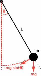
While this post is largely concerned with double pendulums, understanding these systems is made a great deal easier with an understanding of a base “single” pendulum. To be explicit, in this work, we are concerned with an ideal simple pendulum, that is, a point mass (m) handing on the end of a massless string of fixed length (L), which is itself fixed at a pivot point.

A pendulums equilibrium position is directly down. This is where the pendulum will sit in the absence of any external forces. We are concerned with how the pendulum will behave when we displace it from this equilibrium. The laws that will govern this motion are newtons laws of motion for rotational systems.

What we wish to do for our pendulum is derive “equations of motion”, equations describing how it will move through time. To do this, we will be concerned with two things. The first of these is the definition of torque τ (the rotational equivalent of linear force):

τ = ||r|| ||F|| sin(θ)

Where r is a position vector of our pendulum, F a force vector being applied to it, and θ the angle of the force. In our pendulum system, these equations will boil down to:

τ = L * F sin(θ)

Where L is the length of the string, F the force of gravity, and θ the angle of the pendulum.

The second of these things we care about in respect of equations of motion are newtons second law of rotational movement which dictates that:

τ = I * α

This law is analogous to the second law for linear systems (F=MA), in which I is rotational inertia (a quality determined from the masses and lengths in our rotational system) and alpha is angular acceleration. In our pendulum system, this implies that, in addition to the above, torque τ will also be:

τ = mL² d²θ/dt²

We can put these two equations for torque together to get:

L * F sin(θ) = mL² d²θ/dt²

 

With some effort, we can reduce this to an equation of motion:

d²θ/dt² + (g/L)sin(θ)  = 0

Ideally, from this equation we’d like to derive an equation for theta directly in terms of time. Unfortunately, for a general pendulum, we can’t do this: the above equation is intractable, and so we must solve with numerical methods. However, specifically for very small theta, we can use the small angle approximation to make the simplifying assumption that sin(theta) = theta, and derive a closed form equation of motion:

d²θ/dt² + (g/L)θ  = 0

which solves to

θ(t) = θ₀cos(ωt)

Which is the equation of harmonic motion, where ω is the natural frequency of motion.

The end consequence of all of these equations are that the motion of a pendulum is a simple periodic swing back and forth which, for small theta is almost harmonic, that is, the restorative force of the pendulum swinging back is directly proportional to it’s displacement from it’s equilibrium.

Double Pendulum and Chaos

Above, we discuss a simple pendulum and note that, despite the lack of a closed form solution, the behavior of a simple pendulum is fairly simple (and almost harmonic in many cases). We can make this system, and especially it’s behavior, much more interesting by attaching a second (simple) pendulum to the end of the first.

The resulting system is still fairly simple, and in many respects our double pendulum system is fairly similar to that of two single pendulums. However, our equations of motion for the double pendulum become significantly more complicated, to the extent we won’t go through the derivation of these equations here, because they will require several concepts out of the scope of this blog post ( there are many examples online however, e.g. [here], this derivation is a popular problem to set undergraduate physics students). We state the equations of motion as:

θ₁‘ = ω₁

θ₂‘ = ω₂

ω₁‘ =−g (2 m₁ + m₂) sin θ₁ − m₂ g sin(θ₁ − 2 θ₂) − 2 sin(θ₁ − θ₂) m₂ (ω₂² L₂ + ω₁² L₁ cos(θ₁ − θ₂)) / L₁ (2 m₁ + m₂ − m₂ cos(2 θ₁ − 2 θ₂))

ω₂‘ =2 sin(θ₁−θ₂) (ω₁² L₁ (m₁ + m₂) + g(m₁ + m₂) cos θ₁ + ω₂² L₂ m₂ cos(θ₁ − θ₂))/ L₂ (2 m₁ + m₂ − m₂ cos(2 θ₁ − 2 θ₂))

 

Where m₂, m₂ and L₂, L₂ denote masses and lengths of the two pendulums, θ₁, θ₂ denote angles and ω₁, ω₂ denote angular velocities, and g denotes gravity. These equations of motion again don’t have a closed form solution, and will require numerical methods to solve.

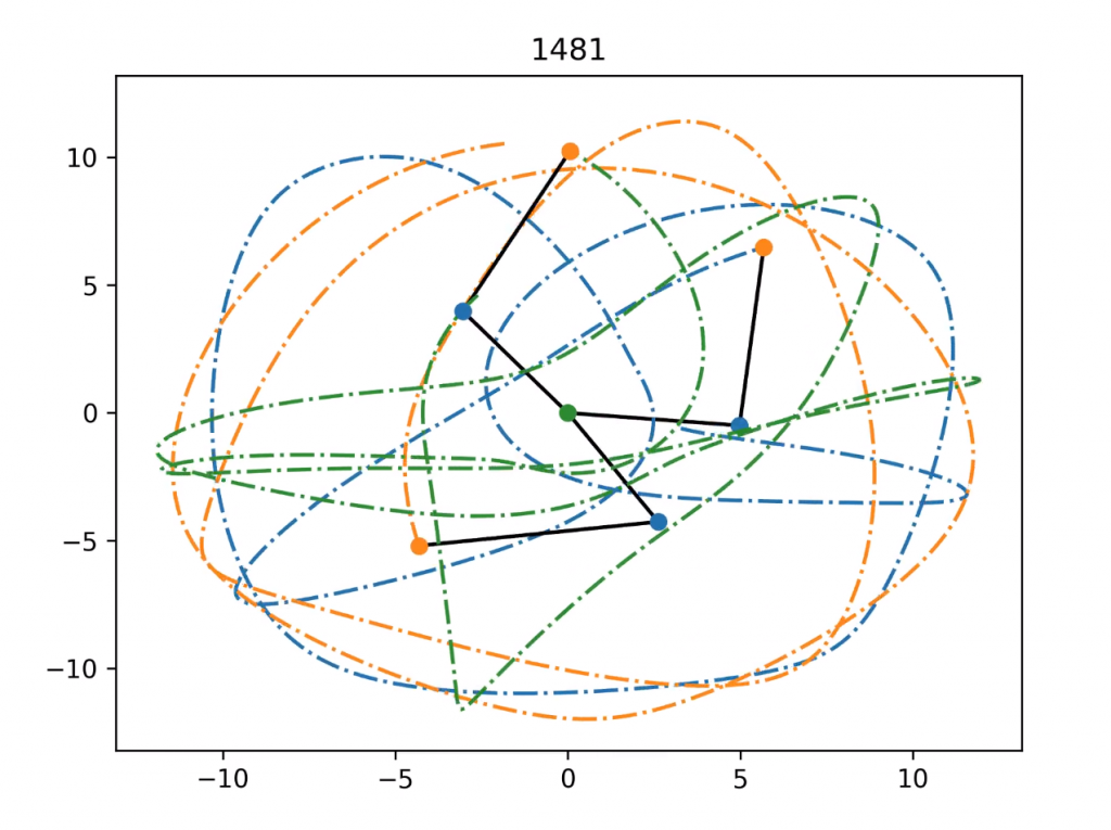
The result of these equations are very much unlike the simple (almost) harmonic motion we observe from a pendulum, and are in fact one of the simplest systems that is often cited as being chaotic.

There’s no one unified definition of chaotic behavior, but typically denote systems whose behavior is highly sensitive to initial conditions (among other conditions). The example animation above displays this well – three different double pendulums starting from almost identical initial conditions ultimately display completely different behavior.