Introduction

I have been exploring the capabilities of the Google Coral development board and working towards a functional face recognition implementation on the embedded device. In a previous blogpost, I discussed an overall view of how the problem might be approached. In this blog post, I dive into more detail on the very first part of a full face recognition pipeline, exposing the different methods of detecting the presence or absence of a face (face detection).

For this purpose, I will be making use of OpenCV (Open Source Computer Vision Library), a machine learning software library that is easy to import in Python. It was quite a challenge to set up OpenCV on the development board, but I can confirm it is possible. You can find the code on my GitHub.

Detection

Face detection is quite a novel technology. It only went mainstream in the early 2000s when Viola and Jones invented a way of detecting faces for low-power devices. As mentioned in the paper, the system was implemented on a device with a low power 200MIPS Strong Arm processor (which lacks floating-point hardware) and still achieved detection at two frames per second.

Since then, a few different methods of detecting faces have been discovered. For my project specifically, I have focused on feature-based methods. What are feature-based methods? They are solutions that rely on a set of training images to output models normally by using features instead of the pixels directly. They rely on techniques from statistical analysis and machine learning to find relevant characteristics of face images. There are many motivations to use features rather than pixels. One of the main reasons is that feature-based systems can potentially operate much faster than pixel-based systems.

Let us discuss briefly what we specifically mean by features, and an example that motivates their use. Most machine learning algorithms typically require a numerical representation of the input to process it and apply statistical analysis. We must reduce our large and/or abstract data into something numeric (and preferably smaller). Feature vectors are the solution. They are used to represent numeric or symbolic characteristics. They are n-dimensional vectors of numerical values that represent some data.

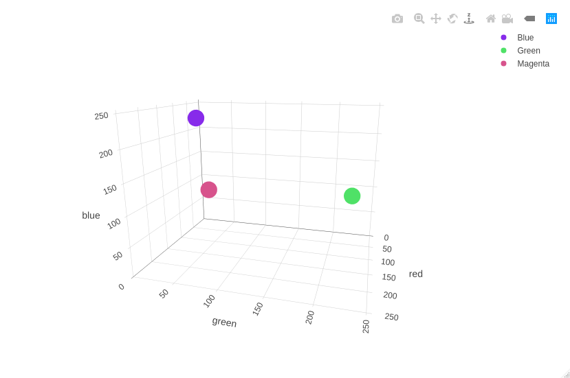
A simple example to explain the need for feature vectors is to apply it to a dataset of colors to check their similarity. To meaningfully classify colors, we need a way of transforming the abstract idea of a “color” to a numerical vector. A way of doing this is by using its RGB (red-green-blue) description. This effectively maps each “color” to a 3 dimensional vector. For example, blue can be represented by its RGB values: [134, 43, 234]. The same can be done to the other colors, meaning that green can be represented as [79, 225, 104] and magenta as [215, 83, 140]. The similar colors (blue and magenta) are close to each other while the colors that aren’t (green and everything else) are further spread out. We can intuitively see this on the plot below. We can see this directly by analyzing their numerical value; we can conclude that blue is more similar to magenta than to green as the difference between their respective vectors is larger.

It is important to keep in mind that this is a very simple example. Often in real-world data analysis, we are not interested in all the information that the sample provides. We want to run computations as fast as possible, thus reducing the size of the data as much as possible is crucial. Additionally, some aspects of our data might not be meaningful, making the samples more complex than they need to be. By using feature vectors to represent data, we can translate abstract ideas to mathematical data in a way that maximizes the “meaningful” portions of the data, allowing us to make use of the vector space to manipulate and modify them.

Below you can see a brief explanation of some of the most popular classification methods for when dealing with faces. Several of the methods are quite famous for those familiar with machine learning techniques (KNN, SVM). The details of these methods are generally related to how the high dimensional space of an image can be compressed down into a reduced space that the classifier can effectively deal with. To cover this fully is a very broad and complex topic that is outside the scope of this blog post, but we aim to give an intuition as to how the problem might be approached by discussing one classified (the Haar Classifier) in more detail.

Classification Methods

Haar Cascade Classifier

A machine learning-based cascade (the term cascade is explained more below). It can run on low-power devices such as mobile phones and cameras. It is a machine learning approach where a cascade function is trained from lots of images, both positive and negative. Based on that training it can be used to detect objects/faces in other images.

Support Vector Machines

Intuitively, the SVM algorithm finds a line that splits the data between the two groups (face/no face, in this case) as well as it can. This line will be such that the distance from the closest point to the dividing line in each of the groups will be the maximal. Previously unseen test cases are classified based on which side of the dividing line they fall. Formally, it attempts to maximize the margin between the decision hyperplane (a flat affine subspace, hyperplane generally) and the examples in the training set.

K-Nearest Neighbour

The goal of K-nearest neighbor (also known as KNN) is to store all available cases and classify new cases based on a similarity measure. Therefore, with KNN you can use the K examples in your dataset that are the most similar to your input to then classify it. A case is classified by a majority of votes from its neighbors, with the case being assigned to the class most common among its K nearest neighbors measured by a distance function (Euclidean for example).

The “K” value is the number of nearest neighbors we wish to take a vote from. For example, if we are classifying handwritten digits and we decide that K = 5 and 3 out of 5 votes for the digit 2, 1 out of 5 votes for the digit 3 and 1 out of 5 for the digit 7 then the algorithm will guess that the unknown input is a 2. The optimal value K varies for different machine learning problems, one way of finding the optimal value of K is by plotting the validation error curve and finding what value of K gives the lowest error.

The Approach

Haar Cascade

This detection algorithm was proposed by Paul Viola and Michael Jones in their famous paper “Rapid Object Detection using a Boosted Cascade of Simple Features” back in 2001. It makes use of a cascade function (something we will explain later), which is trained on a lot of positive and negative images (where positives are those where the face is present, negative when it isn’t). OpenCV offers pre-trained algorithms organised in categories (eyes, faces, etc) saving yourself from having to train your classifier.

The Viola-Jones implementation has four main stages: feature selection, creating integral images, boost training and then finally classifying. The Haar classifier first collects a large number of pre-specified features, however, most of them are irrelevant. To reduce this large number of features, a slightly modified Adaboost then selects the best features and trains the classifier to use them. The Haar classifier works similarly to the convolution kernel but instead of the values of the kernel being determined by training, they are manually set. Therefore, it picks a location from the image, crops a sub-image with the selected pixel as the centre and runs different filters over that space trying to localise a face.

How it works

The idea is that the Haar Cascade extracts features from images using some sort of filter. These filters are called Haar features and look similar to this:

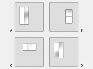
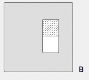
These are rectangle features shown relative to the enclosing detection window. The sum of the pixels which lie on the white area is subtracted from the sum of the pixels in the dark area. As you can see, A and B are used to detect edge features while C detects line features and D four-rectangles features. (Source: Rapid Object Detection using a Boosted Cascade of Simple Features, Viola and Jones, 2001)

The idea is to inspect each area of an image at a time. Then for each area, a single value is obtained by subtracting the sum of pixels under the white rectangle from the sum of pixels under the black rectangle. Ideally, a great value of a feature means it is relevant. Below you can see a very simple example of how the filters are applied:

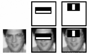
The two features on the top row are overlaid on the training face in the bottom row. As you can see, the first feature is used to measure the difference in intensity between the area around the eyes and the upper cheeks as the eye region is often darker. The second one compares the intensity in the eye region across the bridge of the nose.

While this is a compelling idea, it’s practical realization is non-trivial. There are three main contributions that make it tractible. Firstly, the cascade that gives Haar cascade its name. Secondly, the determination of which features are meaningful and which aren’t. Lastly, a solution to improve slow feature evaluation.

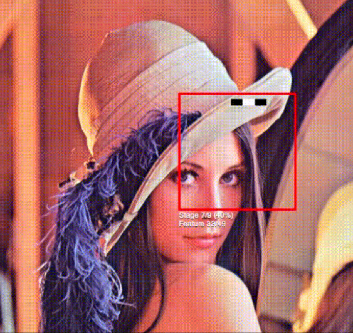
I’m going to briefly address the first contribution, cascading, as it is quite simple. Cascading is a method for combining successively more complex classifiers in a cascading structure, leading to a dramatic increase of speed of the detector by focusing attention on promising regions of the image. We know that if a sub-window doesn’t perform well in a simple classifier it won’t perform well on a more complex classifier. Cascading means that we won’t apply a more complicated classifier to a sub-window until a simple classifier works well. Thus, cascading ensures that we aren’t spending resources on insignificant sub-windows as they will never get to the more complex classifiers. You can see it working below:

The second issue that is going to be addressed is how to determine which features are meaningful. How can we decide which features are relevant out of possibly over 160,000? The answer relies on Adaboost, which selects the best features and trains the classifier to use them. Below you can briefly see the differences between an irrelevant and a relevant feature.

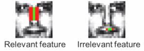
As you can see, feature detecting a vertical edge is useful to identify a nose but irrelevant when detecting lips. (Source: Haar cascade Face Identification – Satyam Kumar – Medium)

Adaboost

The way boosting works is by constructing an ensemble of learners by providing a weak learning algorithm with iteratively modified training datasets, putting increasingly greater weights on the examples deemed more difficult as iterations process. Therefore, it is a method of producing a single very accurate classifier by combining rough and moderately inaccurate classifier.

Adaboost is a popular boosting technique that combines multiple “weak classifiers” into a single “strong classifier”. It specifically trains a set of weak classifiers, such as decision trees. They are considered weak because by themselves they are not meaningful; they are only slightly better than random guessing. Initially, all the training examples will have equal weights. At each step, we use the current weights, train a new classifier and use its performance on the training data to produce new weights for the next step. We keep all the weak classifier as when we are testing on a new feature vector, we will combine the result from all the weak classifiers. An example of a weak classifier might be trying to classify a person as male or female based on their height. You could assume that anyone over 5’9″ is male and anyone under that a female. This way, you would misclassify a lot of people, but the accuracy will still be greater than 50%.

Overall, there are two main things that Adaboost does:

Helps to choose the training set for each new classifier that you train based on the results of a previous classifier.
It determines how much weight should be given to each classifier’s proposed answer when combining the results.

A more abstract example is to compare it to human specialisation. Get a person (weak learner) A to learn problem X. Whatever part of X A is not good at, get person B to learn that subset. Whatever A and B are not good at, get C to learn that. And so on. Each learner specialises in the weakest area the needs the most improvement.

Regardless of how well we solve the feature selection problem, we are left with the difficulty that some features will be slow to evaluate. When scaling the problem, for example by using a 24×24 window, the results are of over 160,000 features. It was quite a challenge back then to make the process of iterating through the whole image efficient. The solution is a concept known as integral image.

Integral Image

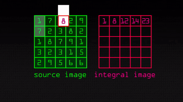
Integral image, very similar to a summed-area table, is an algorithm for quick and efficient computation of the sum of values in a rectangle subset of a pixel grid. The value at any point (x, y) in the integral image is the sum of all the pixels above and to the left of it. After applying integral image, we now only need to refer back to the rectangle corner points and the coordinates of the point separating the white and black region. Furthermore, with just six location references we can find the area of two adjacent rectangles. We can conclude that it is very computationally efficient as it decreases the number of operations needed to find all the sum of the pixel intensities in the specified black and white region (Haar feature).

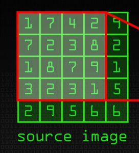
We know that images are simply a matrix of pixels with values ranging from 0 to 255. Therefore, let’s consider the source image below as the input:

(Source: https://www.youtube.com/watch?v=uEJ71VlUmMQ)

We are trying to find a face, thus we want to calculate the area of the rectangle minus another rectangle to find features, like this:

So if we apply this feature extractor to the top left corner we would get 1 + 7+ 7 + 2 – (1 + 3 + 2 + 8) = 3. But if you are doing this over large sections of the image and thousands and thousands of times, it is not going to be efficient. This is where integral image helps. The way it works is if we do one pass over the image, every new pixel is the sum of all the pixels above and to the left of it including it. You can see it intuitively below: